Previously on the blog, Dr Richard Dunley looked at a number of ways that our catalogue, Discovery, can be used as a data source in its own right. Catalogue as Data: the basics explained that if readers want to do detailed analysis of records, they can export search results from the catalogue as a CSV file and open them in Excel or OpenRefine. This allows you to be able to sift the data so as to find out things like ‘what is the geographical spread of this data?’ Or ‘who were the records addressed to?’
In this post I’ll look at how this process can be automated through the Discovery API. To follow this blog, some prior knowledge of coding and machine processing will be necessary.
What is an API?
An API is an acronym for ‘Application Programming Interface’. The Discovery API allows you to do things like filter large sets of data more quickly and reliably than using manual methods in Excel (using code to obtain and analyse the data also reduces the likelihood of manual processing errors while working on the data) and makes it much easier for others to review and replicate that work. The dataset you request is also returned directly in a format that’s useful for machine processing (typically JSON or XML) rather than initially returning a web page that gives you the option to request the data in another format (as Discovery’s ‘Advanced Search’ does).
How do I use it?
To make things easier, we have provided the Sandbox, which is a webpage that gives a simple way to manually enter a set of parameters to send to the API and to see the data returned, along with the exact URL that was used for the API call. This ‘halfway house’ is useful for initial experimentation (without writing code) to understand the sort of data you’ll get back and the filters you can apply. We can then build on this understanding to develop our own code for calling the API directly and for processing the data that it returns to us.
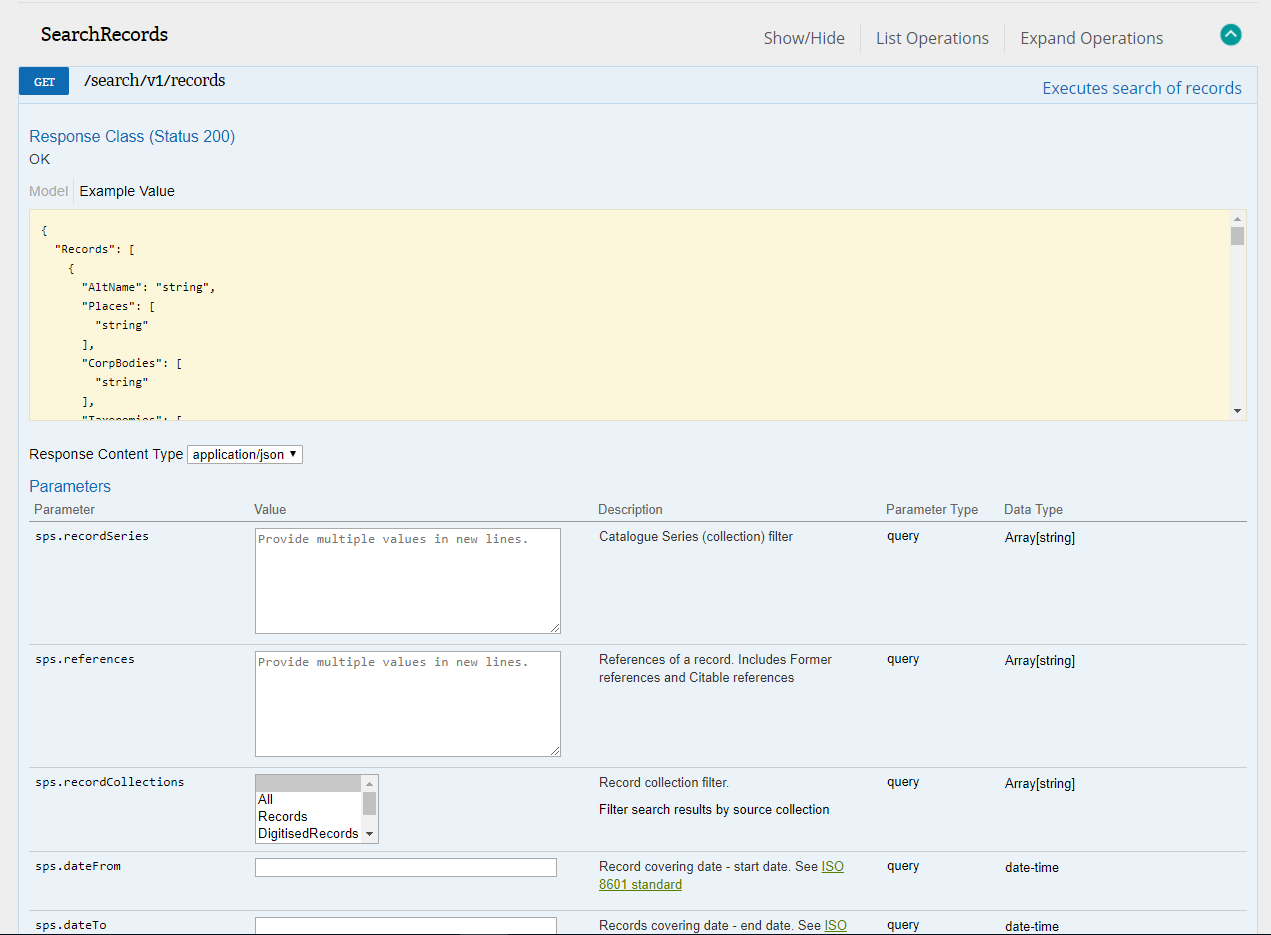
Just as there are several different ways to search or browse Discovery, the API offers several ‘endpoints’ which require different parameters to return data about different aspects of Discovery. The data we want for these experiments is provided by the ‘SearchRecords’ API endpoint. To begin experimenting with this, go to the Sandbox page, and click on ‘ExpandOperations’ in the top right hand corner of the page. You should see something like the screenshot below (all the images in this post can be clicked on for a larger view):
The parameters you can enter on this screen correspond to more familiar things on the normal ‘Advanced Search’ screen in Discovery, although the naming can be a little bit different. For example there are seven ‘levels’ in the catalogue, ranging from ‘a department’ through to an ‘item’ – more information about the catalogue structure can be found here, within the API we use the levels rather than the names as within advanced search.
To make this process easier to follow, I’ll use series SC 8, one of the first examples from Richard’s blog. SC 8 is a series of petitions addressed to the King, the council or other officers of state focusing mainly on the later medieval period. This is a good data set for us to work with as they have been catalogued with a considerable level of structured detail for each petition.
Here’s what we’ve entered within the fields we need:
- sps.recordSeries – we’ve entered record series ‘SC 8’ here, so that it restricts the search to this record series (you could provide several references if you wished to search across different series, each on its own line within the box, hitting <enter> between each).
- sps.dateFrom – for this experiment, we don’t want to pull any data before 1 January 1360, so we’ve set it to 1360-01-01.
- sps.dateTo – we want to restrict the data to 31 December 1380, so we’ll set the ‘dateTo’ to 1380-12-31.
- sps.catalogueLevels – this refers to the ‘type’ of record you want to pull. For this exercise we’d like items only, set this field to ‘Level7’. If you’d like ‘pieces’, you would restrict the search to ‘Level6’.
- sps.sortByOption – we’ve selected ‘REFERENCE_ASCENDING’ to sort the records by reference
- sps.searchQuery – this is the only mandatory field. As we want all items in the series between the applicable dates specified above, we can set this to an asterisk (otherwise known as ‘the wildcard value’). If you were actually only interested in the petitions relating to Lancashire, say, you could put that in as a search term, or anything else that would be relevant to your specific research question.
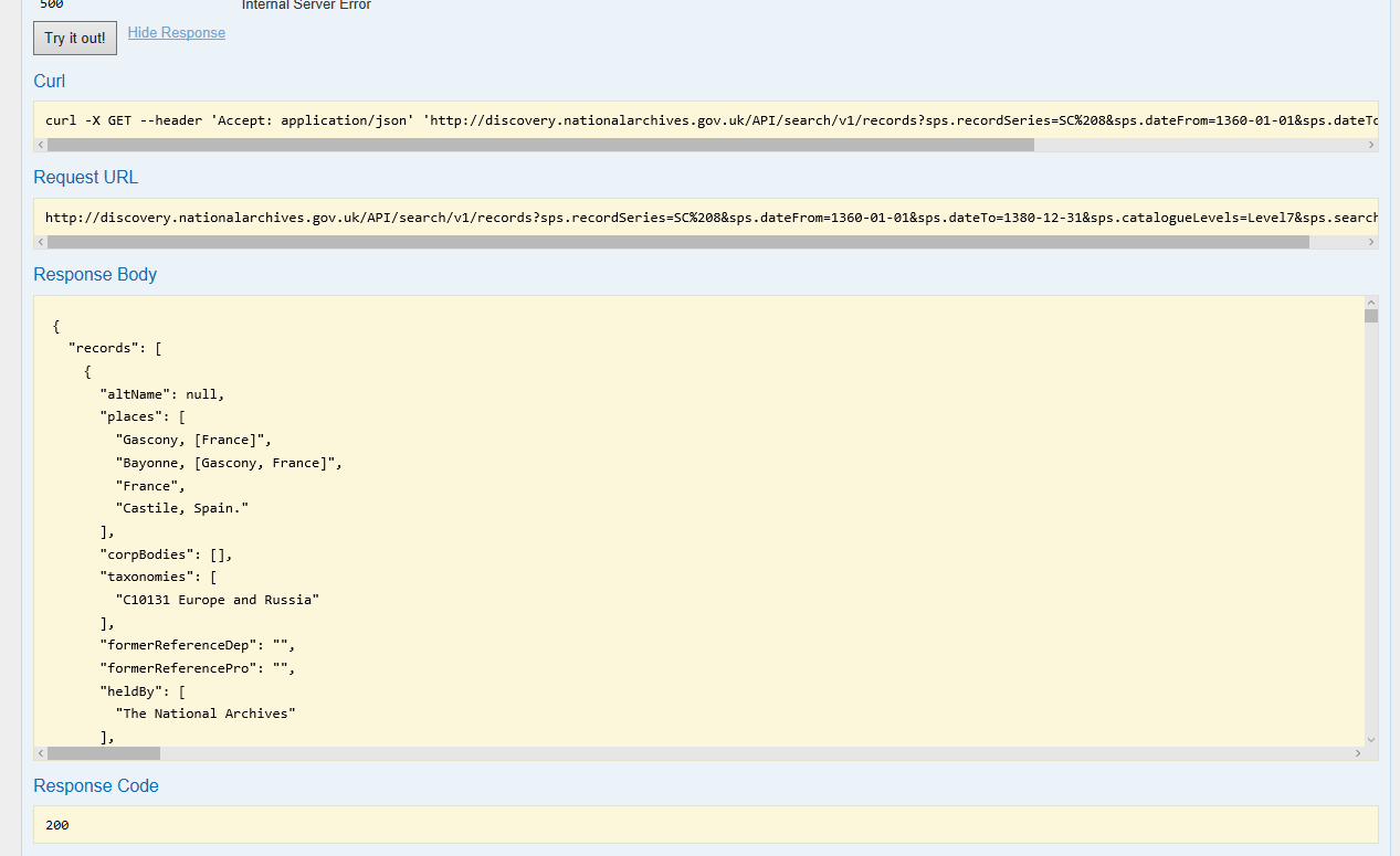
If you just click the ‘Try it out!’ button at this point, you should then see the field below this section, called ‘Response Body’, filled out with the response from the server. The ‘Curl’ and ‘Request URL’ show how you put together calls to the API in a way that programming languages will understand (illustrated in the screenshot below):
How do I see all the data?
If you click into the ‘Response Body’ box and scroll to the end of the data returned you’ll see, "count": 1795.
However, if you look through the earlier part of the Response Body to see how many separate parts you have (each within {} and starting "altName") following "records" you’ll see only 15. How do we get the rest of the records? One of the other parameters available through the endpoint is sps.resultsPageSize, described by the Sandbox as ‘Search results page size. Range [0, 1000], default 15’ – so we’re only seeing 15 because that is the default number of records returned. You can set this to 1000. If you need to see more data, there are a couple of options. There’s sps.page, where you just enter another page number, and you’ll get another page of results, but then you have to work out how many pages there will be based on the count returned by your first call and the page size you specified. The other option is to use sps.batchStartMark. The description says: ‘Cursor Mark value. Search result batch start mark used for deep paging. To invoke deep paging use the ‘wild card’ (*). For subsequent requests use the value of ‘NextBatchMark’ field.’ So what happens if we put an asterisk in this field and ‘Try it out’?
In the Response Body you should see:
"NextBatchMark":"AoI6c2MwMDAwMDAwODAwMDAwMDE1MDAwMDA3MzUoQzkwNjA4NzY=".
Copy the above value and paste it into sps.batchStartMark (without the quotation marks) and ‘Try it out!’ again. If you’ve changed sps.pageSize to 1000 you’ll see that the second set of results you get back return the same value for NextBatchMark. If you left it as the default, that will take rather longer to reach as you get 15 results at a time.
So, if we now look at the ‘Request URL’ we’ll be able to see how these parameters are reflected in the construction of the URL. The ‘base URL‘ is followed by a question mark, then a parameter name followed by an equals sign and then a value, then an ampersand and another parameter and so on. Parameter values have to be ‘URL encoded’: some characters have special meanings in URLs, or are not allowed – those characters have to be converted to a different form to work – so in the URL you’ll see sps.recordSeries=SC%208. Here %20 is the encoded form of the space character, so decoding it, we see that the series is SC 8 as we’d expect.
Automating API usage
Now we just need a way to create such a URL call easily. We ultimately want to base it on some parameters that we pass into a programme, so that the example given here using SC 8 can easily be extended to whatever records series are of interest to you.
I’ll be using the programming language Python 3, which provides good built-in support for manipulating textual information, and a wide variety of packages for simplifying tasks such as accessing APIs and carrying out data analysis. If you’re more familiar with other languages it should be easy enough to see how the general principles could carry over.
The code examples in this post use very basic Python, which should be reasonably straightforward to follow without any prior knowledge. If you’d like to actually learn Python, try the Python Intro for Libraries. I’ve also packaged up my final version of the main script so that it should run as a program on any Windows machine without any installation (or needing to understand the underlying code) – here is the readme file.
In the code examples below, anything to the left of an equals sign can be thought of as just a name which can be used to refer to the things on the right. The only Python-specific things are dictionaries and lists. In the first code example below, myparam is a dictionary, defined by using the curly brackets {} to enclose all its elements, and each element comprises a key:value pair. In this instance the keys are the parameter names, and values the associated parameter values which we will send to the API. To refer to an individual value you use the dictionary name combined with the relevant key, for instance myparams["sps.recordSeries"] would refer to the individual value ['SC 8']. Here the square brackets [] indicate that the value is actually a list, albeit a list containing just a single value of its own in the example. However, as noted above, you can send a list of several series references to the API to indicate that you wish to search within all of them, so if we were doing that you might have something like ['SC 8','WO 95','ADM 362']. There are some further explanatory comments in the code examples, each preceded by #.
Fortunately the third party Python module, Requests, is specifically for making this type of API request very straightforward (among other things). Using this library we can accomplish the basic API call in very few steps, using the following Python code:
import requests;      #version 2.18.4, used for connecting to the API
myparams={"sps.recordSeries":["SC 8"], "sps.dateFrom":"1360-01-01", "sps.dateTo":"1380-12-31", "sps.catalogueLevels":"Level7", "sps.searchQuery":"*", "sps.sortByOption":"REFERENCE_ASCENDING", "sps.batchStartMark":"*", "sps.resultsPageSize":1000};
headers={"Accept": "application/json"}; #we want the API to return data in JSON format
url="http://discovery.nationalarchives.gov.uk/API/search/v1/records";
s=requests.Session(); #creating a session just groups the set of requests together
r=s.get(url, headers=headers, params=myparams); #send the url with our added parameters, call the response "r"
r.raise_for_status(); #This checks that we received an http status 200 for the server response
#so we know nothing's gone wrong with the call (if something has gone wrong we'd get a 404 or 500 error for example)
rjson=r.json()
This will bring back the first page of results from the API as JSON. Using r.json() converts this to a native Python representation as nested lists and dictionaries. To prove this you can look inside the rjson object, and (for example) print out the record count returned:
print("Total records to be retrieved:",rjson["count"])
Now we need to make further calls within a loop to bring back any further pages of results:
while (myparams["sps.batchStartMark"] != rjson["nextBatchMark"] and myparams["sps.batchStartMark"] != "null" ) :
    ## Update the parameter set with the returned value for nextBatchMark so we can get the next portion of data with our next request

    myparams["sps.batchStartMark"]=rjson["nextBatchMark"]

    ## Make our next GET request

    r=s.get(url, headers=headers, params=myparams);
We should again do checks that the call was OK, and get the JSON object containing the next page of records.
Data preparation
We could work with the data in this form, but to do some initial checking and analysis I thought it would be useful to convert the data to a CSV or Excel file to make it easier to compare with the data Richard originally produced. There are a few different ways that I could have done that, but as I also knew that I would need to work on each record to split the description into its constituent parts I opted to use Pandas, the Python data analysis library.
The first step is to create what Pandas calls a dataframe. This is roughly equivalent to a worksheet within a spreadsheet, and in a similar way to a spreadsheet you can refer to the rows and columns of the dataframe, or to an individual cell containing data. When we create the dataframe, we can also (as Richard described in his original blog post), drop the fields that we’re not that interested in, focussing only on the citable reference for each record, the covering date, and ID. In the JSON representation of the data, covering date is actually represented in several ways, to make it easier to work with the dates programmatically, so I’ve kept all of those, and the places mentioned have already been separated out as an individual field as well as being mentioned within the description. So to create the dataframe (which we’ll call ‘df‘) we need a minimum of Python (assuming we’ve joined up all the JSON returned by the API calls above into a single variable called ‘myRecords‘):
import pandas;

df=pandas.DataFrame(data=myRecords,columns=["reference","coveringDates","startDate","endDate","numStartDate","numEndDate","description","id","places"]);
Now we need to do the work of splitting the description column into the individually labelled portions of text. I opted to do this using regular expressions – regex (Richard gave links to some resources for learning regex in his more recent blog post, Catalogue as data: hacking the paper). Essentially, the description comprises a set of labels:
- ‘Petitioners:’,
- ‘Name(s):’,
- ‘Addressees:’,
- ‘Occupation:’,
- ‘Nature of request:’,
- ‘Nature of endorsement:’,
- ‘Places mentioned:’and
- ‘People mentioned:’
Each of these are followed by the related text that we are interested in, for example:
(Petitioners:( )?(?P<petitioners>.*?)\. )?
This separates out the text following a label (here ‘Petititioners‘), and creates a ‘named group’ (using the label text as the name) that we can then use to refer to that section in the Python code that follows. This approach works for this record series but for some other series, such as WO 372 (the First World War medal index cards), where each label can appear more than once for a record, it wouldn’t be as useful. Now we use the Pandas apply function to run the regex against each description in turn, and then put each matching labelled segment into a new column (named for the relevant label) in the dataframe. Next, we can save a CSV or native Excel file using the Pandas to_csv() or to_excel() methods. I also added some checking to verify that text relating to at least one label had been found for each record: there were a couple of cases where nothing was found, for example SC 8/169/8427. I reported these to the Digital Documents helpdesk and the descriptions have now been corrected.
At this point I could have considered the script finished, but I decided to make it more general so it could easily be used for other record series. The final version of the programme can be found in my DiscoveryAPI repository on GitHub. This allows a user to provide input to the script in the form of a CSV file. In that you specify the various parameters for the API, along with a list of the labels you expect to find in the catalogue description (a regex will be automatically constructed from the list), or a specific regex of your own, a file path to save the output to, an Excel sheet name if you specify an Excel file (.xlsx or .xls) in the previous field, a text encoding to use, the data fields from Discovery to include in the output (otherwise this will default to the fields given above) and finally, a maximum number of records to get back from the API (this can be useful when first exploring a record series to prevent a run of the script taking too long). To run the script in its basic form you would need Python 3.6 installed on your own machine, alternatively you can find a .exe at https://github.com/DavidUnderdown/DiscoveryAPI/releases which should run on any Windows machine without the need to install anything (unfortunately I didn’t have any other types of machines available for alternative builds).
Data analysis
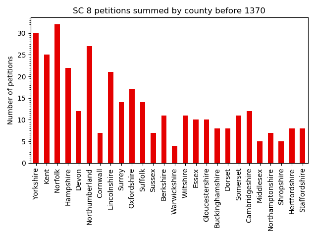
I also wanted to try out recreating the analysis that Richard then performed, again using Python (of course I could have just saved the output as Excel and performed the analysis there). I was less familiar with this aspect of the Pandas library, particularly plotting. After realising that for the plot by counties it was simplest to ask Richard what list of counties he used, I was able to recreate those plots, but a lot of fiddling with options was required to get the axes titles to show nicely without being cropped. The code and plot outputs are in my discovery-data-analysis repository on GitHub.

SC 8 petitions before 1370 summed by county
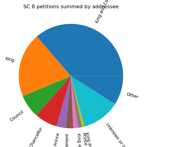
The pie chart proved harder. I worked out the analysis, but trying to get the legend to show for the chart without overlapping the chart itself, or being cropped, has so far proved beyond me. It was also hard to be sure that I had normalised the addressees in the same way that Richard had, so I could not match his results exactly. One advantage of doing the analysis and plotting in code is that anyone else can see exactly what I’ve done and reproduce it exactly. If anyone can fix my plotting output, a pull request would be gratefully received! The first chart was created using the the SC_8_analysis.py file as at commit 0907c5a, while the second and third used the code as at commit 9f977b7.

All SC 8 petitions summed by addressee, showing the problem apparent when labelling the sectors
The examples in this post, along with the code available on GitHub, demonstrate how to make use of the Discovery API to move beyond the advanced search and download capabilities of the Discovery web interface. I’ve released the code under an open licence (the BSD 3-clause License) so they can be used as a starting point for anyone who would like to use them in looking at their own research questions.

